How to Create a Pivot Table in Microsoft Excel | 6 Methods to Try

Pivot Table is an awesome element of Microsoft Excel. With its help, you can summarize large complex data in a simplified manner. The functionalities of Pivot Table are just amazing to use. I know you might be thinking it is difficult to make a Pivot Table. To make it easier for you, I have written it in the simplest form. So, what are you waiting for? Start reading the entire article on how to create a Pivot Table in Microsoft Excel.

If your boss has given you complex numerical data, you might have started feeling frustrated to see the big complex data. Worry not, you can create it easily and get it done on time. For this, Microsoft Excel gives you amazing features to create a Pivot Table so that you prepare an awesome report.

If you are eager to know how to do it, quickly read the subheadings below. This will help you to arrange all types of data. Open your excel sheet, and start applying the steps to summarize your data.

How to Create a Pivot Table in Microsoft Excel Instantly?

A Pivot Table is a powerful tool for calculating, summarizing, and analyzing the data, allowing you to identify similarities, designs, and trends.

If you have a large data that you created on the Excel sheet, you can create a Pivot table to arrange the data. To know how to create a Pivot Table, follow the steps below-

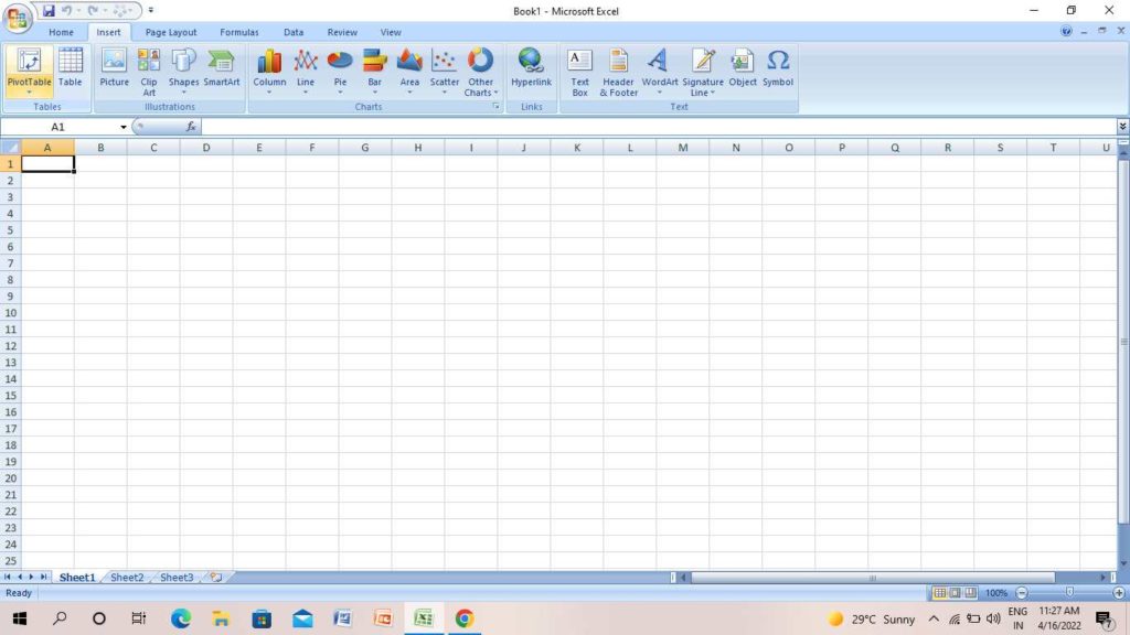
1. Create data on the Excel sheet.
2. On the home screen, tap on Insert.

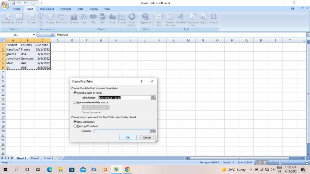
3. Create Pivot Table window will appear on the screen,

4. Tap on Ok.

5. On the right side of the screen, the PivotTable Field list will appear.

6. Drag the fields in different areas like Report Filter, Column Labels, Row Labels, and Values.

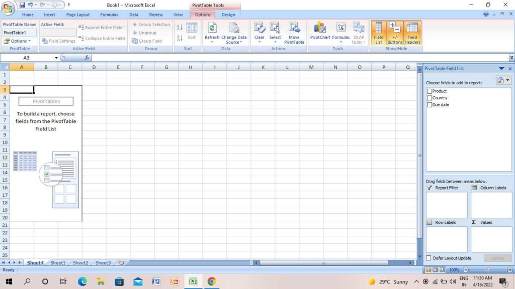
Pivot Table will appear on the screen with the adjustment of the fields in different areas.

How to Create a Pivot Table in Microsoft Excel | Apply Sort

If you want to sort any data on the top of the list, you can do it with the help of the Sort function. To know how to do it, follow the steps below-

1. Go to the data that is on the column of the Pivot table.
2. Right-click on any cell.
3. Tap on Sort.

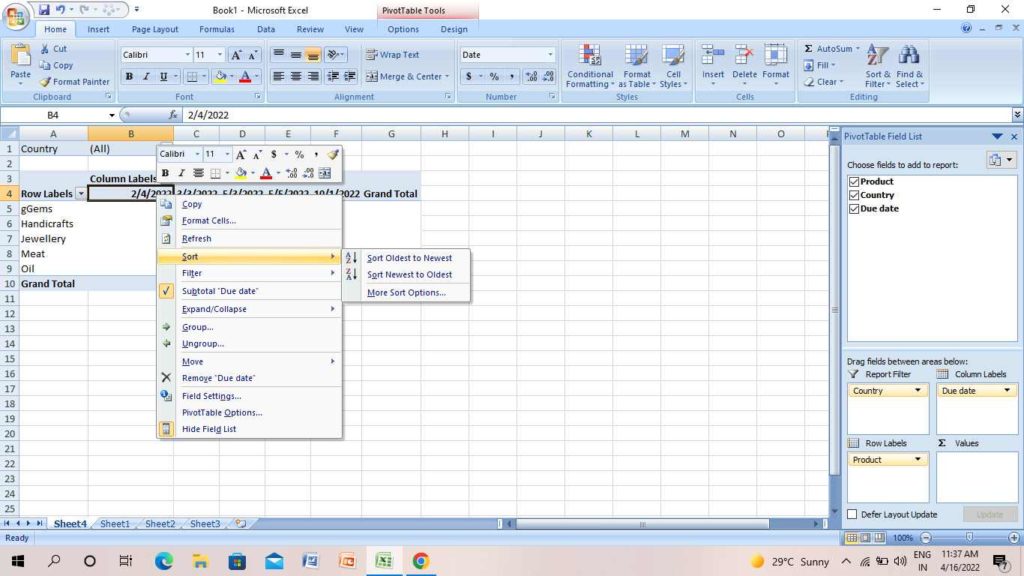
4. Tap on any option like Largest to Smallest, A to Z, or others.

How to Create a Pivot Table in Microsoft Excel | Use Filter

To select a particular data in the Filter area, you can easily o it on the excel sheet. To know how to do it, follow the steps below-

1. On your excel sheet, tap on the Filter area on top.

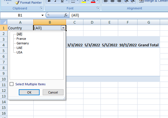
2. In the drop-down menu, select the option.

3. Tap on Ok.

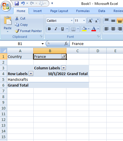
Thus, you will see the results will appear on the screen on your Pivot Table.

How to Create a Pivot Table in Microsoft Excel | Change Calculation

There is also an option on the Pivot table that will help you to change the calculation default setting of the Pivot table. The default calculation setting is either sum or count. If you want to change it, follow the steps below-

1. On the Amount cell, right-click on it.
2. Tap on Value field settings.

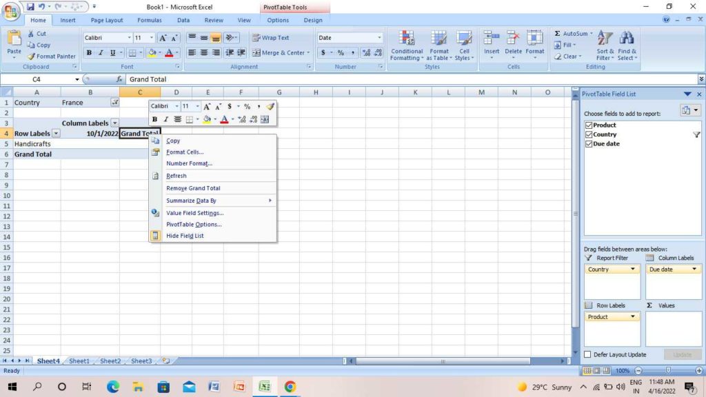
3. On the next window pop-up, go to the Value field.

4. Select the calculation that you want.

5. Finally, tap on Ok.

How to Create a Pivot Table in Microsoft Excel | Two Dimensional Pivot Table

If you want to create a two-dimensional Pivot Table, you have to follow a few steps, and the results will appear instantly. To know how to do it, follow the few steps-

1. Select the area in the PivotTable fields.
2. Drag the fields to different areas.

For example, drag Country to the Rows area.

                    Due Date to the Column area.

                 Products to Filter area.

                    Amount to Values area.

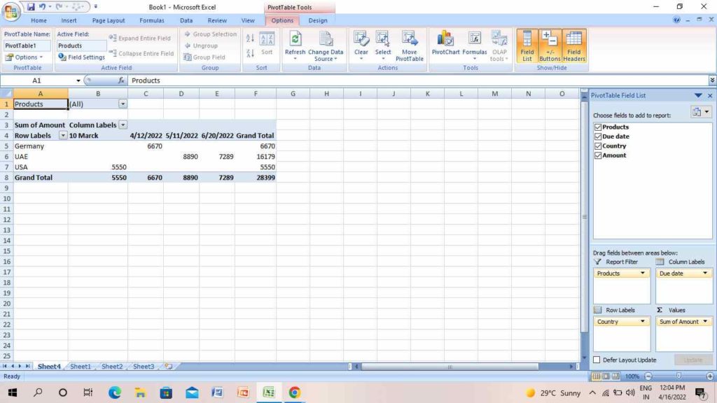
Thus, you will see the results will appear on the screen on the Pivot table.

How to Create a Pivot Table in Microsoft Excel?

If you want to know how to create a Pivot Table in Microsoft Excel, follow the step-by-step guide in the below video. To know how to do it, follow the steps below-

How to Create Pivot Tables for Dummies?

If you are confused about how to create Pivot Tables for Dummies, just follow the instructions in the below video and create it instantly.

Wrapping Up

Thus, with the use of the above steps, you understand how to create a Pivot Table in Microsoft Excel. You can create the Pivot table and arrange the data accordingly. Feel free to share the article with your friends. Now, it is time for a wrap-up. Stay tuned for all the exciting updates. Have a great day!

Frequently Asked Questions